Tuesday, February 27, 2007

9.1 Modeling with Differential Equations

Alright, so in class we learned about the two different models of population growth. The first one is stated as the Rate of Growth for a Population-unbounded on our concept sheets. It is:

This equation shows that population is always growing, and as it gets bigger its growth rate gets bigger as well. As Mr. French said, as the population gets bigger, there's more people to make the population bigger.

The second formula we were taught is dubbed the Rate of Growth for a Population-bounded on our concept sheets. It is:

This equation is also the derivative of a logistic function. It expresses the fact that when we have a small population, the population will grow quickly. But as the population approaches the carrying capacity, it won't be able to grow so quickly and will level off. If P/K were to ever become greater then 1, then the population would start to decline.

The next thing we learned about was the IVP, or the Initial Value Problem. The two steps to these situations are:

1. Solve the differential equation for a general solution.
2. Use the general solution and data point to solve for a specific solution.
For example:

Given and the point y(0)=5, find the IVP.


http://www.math.ohiou.edu/~ashish/h13.pdf That's a nice quick summary straight from our book that Ohio University made.

http://www.mathsci.appstate.edu/~hph/3310/diffeqn/ This site has examples of different kinds of differential situations.

Alex, you get the blog next =D


My favorite quote for the past month has been "You smell funny" from POTC:DMC.


And now for some lame math jokes...


Q: What is the first derivative of a cow?

A: Prime Rib!


Q: What caused the big bang?

A: God divided by zero. Oops!


"A mathematician is a blind man in a dark room looking for a black cat which isn't there."- Charles Darwin


and for my last few words:


A guy gets on a bus and starts threatening everybody: "I'll integrate you! I'll differentiate you!" So everybody gets scared and runs away. Only one person stays. The guy comes up to him and says: "Aren't you scared, I'll integrate you, I'll differentiate you!" And the other guy says: "No, I am not scared, I am e^x."

Thursday's Quiz Topics

Here’s a list of topics that will be covered on this Thursday’s Quiz.

Quiz – Sections 8.1, 9.1
Arc length – given curve and interval (8.1, #1,3,5,9,11,29)
Arc length – determine setup (8.1, #1,3,5,9,11,29)
Arc length – given curve and interval (8.1, #1,3,5,9,11,29)
Arc length – given curve, determine interval (8.1, #1,3,5,9,11,29)
Differential equation – analysis and interpretation (9.1, #11)
Differential equation – verification of solution (9.1, #1,5)

That’s it for now! I’ll be around after school on WEdnesday and online Wednesday evening/night.

In any collection of data, the figure most obviously correct,
beyond all need of checking, is the mistake

Corollaries:
(1) Nobody whom you ask for help will see it.
(2) The first person who stops by, whose advice you really
don't want to hear, will see it immediately.

And on another note, look for the simple solution:

Monday, February 26, 2007

8.1 Arc Length

Okay, so it's finally my turn again~! I'm here to explain Chapter 8, Lesson 1, which is about finding arc lengths.

When a curve is a polygon, finding the length is easy because all you have to do is add up the sides but when you get a continuous curve, it gets tricky! Remember that a curve is defined by the equation y= f(x) where f is continuous on a (equal to or less than) x (equal to or less than) b. When we estimate the value of a curve, we are taking approximations as if the sides of a polygon were present in it. (page 547 in the textbook)

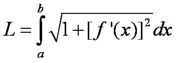
The length is described using the distance formula (as the limit approaches infinity). The distance formula is not practical to use with a smooth function, so we can derive an integral formula for L where the function has a continuous derivative, because there is only a very small change in f'(x). (Also think of the approximation as taking the Pythagorean theorem to find the hypotenuse with infinitely many tiny triangles, as described in class)

The arc length forumula for the curve y=f(x) where is a is (equal to or less than) x (equal to or less than) b

(if f' is continuous on [a,b])
Photobucket - Video and Image Hosting
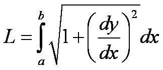
it can also be notated as:
Photobucket - Video and Image Hosting

In the other case, if a curve has the equation x=g(y) with c (less than or equal to) y (less than or equal to) d, and g'(y) is continuous, we get this formula for arc length:
Photobucket - Video and Image Hosting


Keeping these two formulas in mind, let us try a problem!

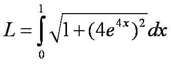
If y=e^4x and 0 (less than or equal to) x (less than or equal to 1), find the arc length.

We begin by writing the integral, which will be from 0 to 1, and plug in the derivative. Remember to use the chain rule in this case, because the derivative of e^4x is 4(e^4x). Don't forget details such as chain or product rule when taking derivatives! Also remember to even TAKE the derivative, and to SQUARE it. But I digress. After setting everything up, it should look like this:

Photobucket - Video and Image Hosting

Afterwards, you can either figure out the antiderivative or if you are short on time or just wish for simplicity (in this case), plug it in to your calculator and do fnInt! Oh yeah, another minor detail. Don't forget to write "dx" when doing your problems, and don't get your dx's and dy's mixed. I think it's just me, but it's still a possible mistake.

...aaaannndddd here are a few links:

http://en.wikipedia.org/wiki/Arc_length (history teachers can scorn Wikipedia but this site gives a good explanation of this math concept, provided that no users/pranksters go edit it, but it always gets edited back anyhow)
http://tutorial.math.lamar.edu/AllBrowsers/2414/ArcLength.asp

http://www.math.hmc.edu/calculus/tutorials/arc_length/


and here's a funny little video for you all. just remember when you decide to bring your kitten in for show-and-tell, don't let it near Mr. French's laptop. (Has anyone posted it on the blog already? Remind me if anyone has)


carpe diem, everyone.

until next time~!

-Sonia

Oh yea, Crystal. You're up next xD

Wednesday, February 21, 2007

Section 7.7 Approximate Integration

Hello everyone.
This section is called Approximate Integration. It covers three methods of approximating integrals, but only two of them are covered on the AP Exam.

The first method is the Midpoint Rule. We have covered this before, but just in case you cannot remember it, here it is:


where (for all of the equations).

This calculates the area under a curve using rectangle approximations, using the midpoints as the heights. A more accurate method is trapezoidal approximation. Instead of drawing rectangles under the curve, you can draw trapezoids. Here is the formula for using trapezoidal approximation.


Finally, there is a third method that is not on the AP Exam, and it is known as the Simpson’s Rule. Here it is:


For this to work, n must be even.

Here is an example:


For use the Trapezoidal Rule, the Midpoint Rule, and Simpson’s Rule to approximate the integral if n = 4.


For the Trapezoidal Rule, plug in the values for the equation. First calculate .


Now:

This method gives us an approximation of 44.


Using the midpoint rule, will be the same. Next find the midpoints.


Now plug into the equation:


This gives us an approximation of 21.Finally, for Simpson’s Rule. remains the same.

Plug into the equation:

This gives us an approximation of .

And that's the lesson.


Here is a link to a helpful resource: This website shows the Trapezoidal Approximation and Simpson’s Rule and how to use them: http://archives.math.utk.edu/visual.calculus/4/approx.1/index.html

Sonia you are next.

On a lighter note, here are some comics:


Friday's Quiz Topics

Here’s a list of topics that will be covered on this Friday’s Quiz.

Quiz – Sections 7.1,7
Integration by Parts – basic (7.1,#3,7)
Integration by Parts – definite integral
Integration by Parts – f and g won’t go away (7.1,#15 - not assigned, but good practice!)
Integration by Parts – tabular method (7.1, #61)
Trapezoidal Rule (7.7, #1,3,7,29)
Midpoint Rule (7.7, #1,3,7,29)

That’s it for now! I’ll be around after school on Thursday (after 3:30) and in early on Friday. Donut holes and OJ...

At New York's Kennedy Airport today, an individual, later discovered to be a public school teacher, was arrested trying to board a flight while in possession of a ruler, a protractor, a set square, and a calculator. Attorney General John Ashcroft believes the man is a member of the notorious Al-Gebra movement. He is being charged with carrying weapons of math instruction.
Al-Gebra is a very fearsome cult, indeed.They desire average solutions by means and extremes, and sometimes go off on a tangent in a search of absolute value. They consist of quite shadowy figures, with names like "x" and "y", and, although they are frequently referred to as "unknowns", we know they really belong to a common denominator and are part of the axis of medieval with coordinates in every country. As the great Greek philanderer Isosceles used to say, there are 3 sides to every angle, and if God had wanted us to have better weapons of math instruction, He would have given us more fingers and toes.
Therefore, I'm extremely grateful that our government has given us a sine that it is intent on protracting us from these math-dogs who are so willing to disintegrate us with calculus disregard.
These statistic bastards love to inflict plane on every sphere of influence. Under the circumferences, it's time we differentiated their root, made our point, and drew the line. These weapons of math instruction have the potential to decimal everything in their math on a scalar never before seen unless we become exponents of a Higher Power and begin to appreciate the random facts of vertex.
As our Great Leader would say, "Read my ellipse". Here is one principle he is uncertainty of---though they continue to multiply, their days are numbered and sooner or later the hypotenuse will tighten around their necks.

Tuesday, February 20, 2007

7.1 Integration of Parts

You should remember that the product rule is :

By rearranging this equation you see that:


By using the substitution rule and replacing u for f(x), v for g(x), du for f'(x)dx, and dv for g'(x)dx, you will see that the formula for integreation of parts becomes:


Let's look at a couple of examples!
1)
Choose your simplest component for u. In this case that would be x. Make a table of your u, du, v, and dv.

Now plug it into the equation
You get


Don't forget the C!

2)
You can use the tabular method here.


Now try a problem!


Here, you must use integration by parts again


Now plug this equation back into the end of the first integration of parts:


Here is a good site for Integration of Parts:
http://www.sosmath.com/calculus/integration/byparts/byparts.html


Saladang Song: My obsession with food has led me to this great Thai restaurant. I highly recommend it (especially the Yellow Curry) and it's very well priced.
363 S Fair Oaks Ave (Cross Street: W Bellevue Drive)Pasadena, CA 91105

Kyle, you're up next!